DIFFERENTIAL GEOMETRY IMAGES
These images
were constructed using the programs in
Modern Differential
Geometry of Curves and Surfaces
with Mathematica (Second Edition)
by Alfred Gray
The Mathematical Legacy of Alfred Gray : International Congress on Differential Geometry September 18-23, 2000, Bilbao, Spain
For a
review of Gray's book (second edition) see
SIAM
Review, Volume 41(1999), No. 1, pages 186-189.
The images and animations below, and
the
Mathematica programs which generate them, are part of
the course
materials for
Introduction to Differential Geometry 1 & 2 at the University of Iowa.
Please email
walter-seaman@uiowa.edu if you would like
additonal information.
Topics list
When you click on the picture, it should
link to the animation.

Click on the picture to see the animated view.
Or right click and choose "Save Target As" or "Save Link As"
here
to download a QuickTime movie (.mov file) of this animation.
Picture/animation explanations:
With the definitions
torus[a, b, c][u, v]
:= {(a + b*Cos[v])*Cos[u], (a + b*Cos[v])*Sin[u], c*Sin[v]}
and torusknot[a, b, c][p, q][t] :=
{(a + b*Cos[q*t])*Cos[p*t], (a + b*Cos[q*t])*Sin[p*t], c*Sin[q*t]}
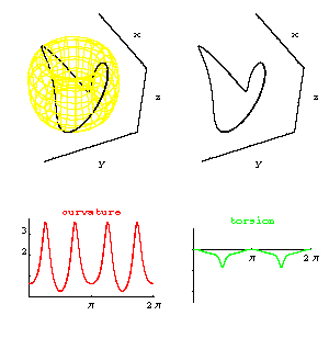
this graphic shows the
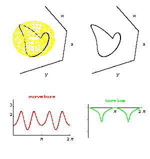
torusknot[8,3,5][1,2][t]
on the torus torus[8,3,5], shown in a yellow wireframe view, along with the curve
alone.
Also shown are the graphs of the
curvature (red) and torsion (green) functions for this curve, graphed over the
t-axis.
Clicking on the graphic runs an animation which is determined by letting
t increase from 0 to 2 pi in increments of 2Pi/20,
for the torusknot curve, its curvature
and its torsion functions.
So in the animation the 'leading edge' of the torusknot
curve has curvature and
torsion values given by the (y-coordinates of the) leading edge of the graphs
of those corresponding
functions.
This graphic also
illustrates 'which' points on the curvature and
torsion graphs correspond to which points on
the torusknot curve, for the given
parameterization.
Back to
Topics list.
Back to top.
<
click and choose "Save Target As" or "Save Link As"
here
to download a QuickTime movie (.mov file) of this animation.
Click on the picture to
see the animated view.
Or right click and choose "Save Target As" or "Save Link As"
here to download a
QuickTime movie (.mov file) of this animation.
Picture/animation explanations:
With the
definitions
torus[a, b, c][u, v] := {(a + b*Cos[v])*Cos[u], (a + b*Cos[v])*Sin[u], c*Sin[v]}
and
torusknot[a, b, c][p, q][t] :=
{(a + b*Cos[q*t])*Cos[p*t], (a + b*Cos[q*t])*Sin[p*t], c*Sin[q*t]}
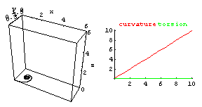
this graphic shows the curvature and torsion for the curve torusknot[8,3,8][1,2][t]
on the
torus[8,3,8], shown in a yellow wireframe view,along with the curve
alone.
Clicking on the graphic
runs an animation which shows how the
torus, the torus knot, and its curvature and torsion change
when we
graph torusknot[8,3,c][1,2][t]
on the torus[8,3,c], and let c vary. We vary c from 5 to 8, then
from 8 to
3, then back to 5.
This animation is meant to
illustrate how curvature and torsion change
when the curve (the torusknot
in this case)
changes in a controlled way.
Back to
Topics list.
Back to top.
Click on the picture to see the animated view.
Or right click and choose "Save Target As" or "Save Link As"
here
to download a QuickTime movie (.mov file) of this animation. Picture/animation explanations:
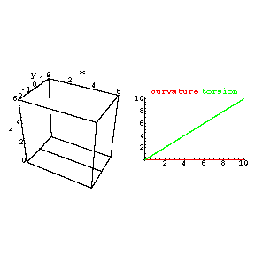
In the right graphic,
the red line is the graph of
Curvature[ t ] = t, the green
line
is the graph of
Torsion[ t ; n ] = n t, with n = 0,
with t in [0,10]. In
the left graphic is the numerically-generated unit-speed space curve
alpha[ t ; n ] with
curvature = Curvature[ t ] and torsion = Torsion[ t ; n ] for t in [0,10].
The initial
conditions for alpha[ t ; n ] are
alpha[ 0 ; n ] = {0,0,0}, t-derivatives alpha ' [ 0 ; n ] = {1,0,0} and
alpha '' [0;n]
is normalized to {0,1,0}.
We then vary n from 0 to 1 in increments of .1 The changes in the curve alpha[ t ; n ] and the
graph
of Torsion[ t ; n ]
are shown in the animated view. This animation gives a 'dynamic' view of what
the torsion of a space curve
controls (how much the curve is
'stretched out'). The alpha[ t ; n ] curve is obtained by
solving the Frenet frame equations
numerically with a program Gray
wrote using the Mathematica function
NDSolve.
Back to
Topics list.
Back to top.
 Click on the picture to see
the animated view.
Or right click and choose "Save Target As" or "Save Link As"
here
to download a QuickTime movie (.mov file) of this animation. Picture/animation explanations:
In the right graphic,
the red line is the graph of
Curvature [ t ; n ] = n t, with n = 0 the
green line
is the graph of
Torsion[ t ] = t, with t in [0,10]. In
the left graphic is the numerically-generated unit-speed space curve alpha[ t ; n ] with
curvature = Curvature[ t ; n ] and 'torsion' = Torsion[ t ] for t in [0,10] (see below
for some remarks about this). The initial
conditions for alpha[ t ; n ] are
alpha[ 0 ; n ] = {0,0,0}, t-derivatives
alpha ' [ 0 ; n ] = {1,0,0} and alpha '' [0;n] is normalized to {0,1,0}.
We then vary n from 0 to 1 in increments of .1. The changes in the curve alpha[ t ; n ] and the
graph of Curvature[ t ; n ]
are shown in the animated view. This animation gives a 'dynamic' view of what
the curvature of a space curve controls (how much the curve
'winds around'). The alpha[ t ; n ] curve is obtained by
solving the Frenet frame equations numerically
with a program Gray
wrote using the Mathematica function
NDSolve.
For n = 0, the curve
alpha[ t ; n ] is a plane curve, even though its 'torsion' is nonzero. This is
because we chose the curvature to be
identically
zero. In this case the function we have called the torsion function does not
behave like the usual notion of torsion, which is
defined when the curvature is nonzero.
One can pick 'any' two (say smooth) functions, K[ t ] and T[ t ] to play the roles of the curvature and
torsion functions appearing in the Frenet frame equations, and a
solution curve to those equations is obtained, C [ t ; K ; T ]
(given initial conditions).
The relation between the 'usual' notions of curvature
and torsion for C [ t ; K ; T ] and K[ t ] and
T[ t ], especially when K[ t ] takes zero or
negative values, is explored in exercises in the course.
Back to
Topics list.
Back to top.
 Click on the picture to see the animated view.
Or right click and choose "Save Target As" or "Save Link As"
here
to download a QuickTime movie (.mov file) of this animation. Picture/animation explanations:
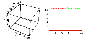
In the right graphic,
the red line is the graph
of
Curvature[ t ; n] = n t, the
green line
is the graph of
Torsion[ t ; n ] = n t, both with n = 0 , with t
in [0,10]. In
the left graphic is the numerically-generated unit-speed space curve alpha[ t ; n ]
with
curvature = Curvature[ t ; n ] and torsion = Torsion[ t ; n] for t in [0,10]. The
initial
conditions for alpha[ t ; n ] are
alpha[ 0 ; n ] = {0,0,0}, t-derivatives
alpha ' [ 0 ; n ] = {1,0,0} and alpha '' [0;n] is normalized to {0,1,0}.
We
then vary n from 0 to 1 in increments of .1 The changes in the curve alpha[ t ; n ]
and the
graph of Curvature[ t ; n ] and Torsion[ t ; n ]
are shown in the animated view.
This animation gives one possible view of what
happens to a space curve when both its
curvature and torsion are varied (a sort
of competition between streching out and winding around!).
Many other choices
of curvature and torsion functions can be examined by minor modifications
to the
program Gray wrote to generate the space curves.
The alpha[ t ; n ] curve is obtained by
solving the
Frenet frame equations numerically with a program Gray
wrote using the Mathematica function
NDSolve.
Back to
Topics list.
Back to top.
Click on the picture to see the animated
view.
Or right click and choose "Save Target As" or "Save Link As"
here
to download a QuickTime movie (.mov file) of this animation. Picture/animation explanations:
This animation
illustrates how certain basic surface parameterizations distort
lengths of curves.
This idea leads to a discussion of intrinsic versus non-intrinsic properties
of
surfaces.
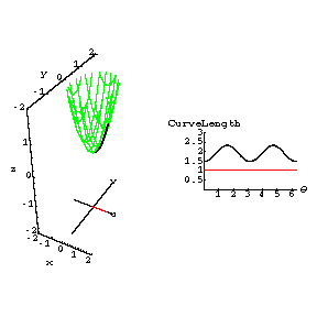
In the
left graphic, the green
paraboloid[1,2][u,v]= {u , v, u^2 + 2 v^2} surface
(in 'wireframe' view) is shown over
the x-y parameter
plane. A copy of the u-v plane is shown the plane z = -1.
In this
plane are red line segments
of length 1 starting at the
point (0,0). The images of these line
segment are shown are thick black curves
on the surface.
In the right graphic the lengths of the curves on the surface are
shown
in black as a function of the 'polar angle' in the plane.
Also shown in
red are the lengths of the original
line segments
(all of which = 1).
Back to Topics list.
Back to
top.
Click on
the picture to see the animated
view.
Or right click and choose "Save Target As" or "Save Link As"
here
to download a QuickTime movie (.mov file) of this animation. Picture/animation explanations:
This animation
illustrates
how certain basic surface parameterizations distort lengths of tangent
vectors.
This idea leads to a discussion of induced metrics on surfaces and on the domains of
the
parameterizing
coordinate patches. Later, this leads to a discussion of
a
metric on a plane domain which may or may not
arise from an embedding
into three-space.
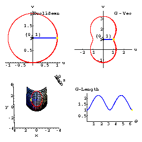
In the upper left graphic, the
blue tangent vectors
with yellow tips in the
u-v plane are based at the point (0,1). These
have length 1
and their endpoints trace out the
red (Euclidean) circle
of radius 1.
These vectors are mapped to the surface
z = x^2 + y^2 by the tangent map to the parameterization
paraboloid[1,1][u,v]= {u , v, u^2 + v^2}. In the
graphic on the lower left, the image vectors
on the
paraboloid[1,1] at the point {0,1,1} are shown in
blue,
and the image of
the circle is shown in red.
The lengths
of these image vectors (labeled G-length
) are shown in the
blue
curve in the lower
right graphic, as a function of the
'polar angle' in the u-v plane.
In the upper right graphic is
shown the original
blue vectors,
now measured with the 'induced metric', that is, with the lengths
given by the
lengths of the images tangent to the surface.
Back to
Topic list.
Back to
top.
Click on
the picture to see the animated
view.
Or right click and choose "Save Target As" or "Save Link As"
here
to download a QuickTime movie (.mov file) of this animation. Picture/animation explanations:
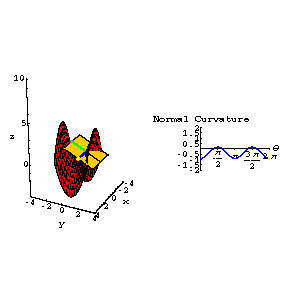
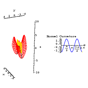
The surface z = y^2 - x^2 is shown in red. The
green 'upward' normal is located at (0,0,0). The normal
curvature is computed in the direction of the blue
tangent vector at (0,0,0).
The blue and green
vectors span the yellow slicing plane.
The normal curvature is (up to sign) the ordinary space curve
curvature of the
curve given by the intersection
of the slicing plane and
the surface. The normal curvature is positive
when the slice curve
'bends up towards' the chosen normal,
and negative when it 'bends down away'.
The intersection curves are shaded black.
It is an exercise in the course to prove that these
curves are the images of straight lines
through {0,0} in the u-v parameter plane
under the parameterization { u , v , -u^2 + v^2 }.
In the right-hand frame the normal curvature
is graphed as a
function of the 'polar angle' of the
blue tangent vector. The 'polar angle' is
defined using the parameterization for a basis of
the tangent space, and applying the Gram-Schmidt
process to that basis.
Explaining this was also part
of an exercise.
Back to Topic list.
Back to top.
 Click on
the picture to see the animated
view.
Or right click and choose "Save Target As" or "Save Link As"
here
to download a QuickTime movie (.mov file) of this animation. Picture/animation explanations:
The surface z = y^2 - x^2 is shown in red.
The green 'upward' normal is located at
(0,1,1). The normal curvature is computed in the direction of the
blue tangent
vector based at (0,1,1). The blue
and green vectors span the
yellow
slicing plane. The normal curvature is (up to sign) the ordinary space
curve
curvature of
the curve given by the intersection of the slicing plane and the surface.
The normal curvature
is positive
when the slice curve 'bends up towards' the chosen normal,
and negative
when it 'bends down away'. In the right-hand frame the normal curvature is
graphed
as a function of the 'polar angle'
of the blue
tangent vector. The 'polar angle' is
defined using the parameterization for a
basis of
the tangent space, and applying the Gram-Schmidt
process to that basis. Explaining this was part
of an exercise in the course.
Back
to Topics list.
Back to top.
Click on
the picture to see the animated view. Or right click and choose "Save Target As" or "Save Link As">
here
to download a QuickTime movie (.mov file) of this animation. Picture/animation explanations:
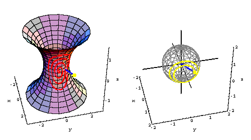
In the left graphic,
the catenoid surface, the surface of revolution
obtained by rotating the catenary curve y = cosh[x] about the x-axis, is shown with
a
red curve on it.
This curve obtained by mapping the
unit circle
centered at the origin of the u-v plane to
the catenoid by the
parameterization
cyl[u,v] = {cos[u]cosh[v],sin[u]cosh[v],v}.
The blue
'outward'
unit normal with a yellow tip is shown at a
point
of this curve.
In the right graphic the blue
unit normal with
yellow
tip is shown translated to the origin,
with its
yellow
tip on a gray
sphere
(shown in wireframe view).The
yellow curve on the sphere is the image of
the red
curve under the
Gauss map of the catenoid. It consists of the image points
of the yellow
tips of the blue
unit
normals as the base points vary about the
red
curve. Note the apparent "reversed" orientations of the normal vectors on the catenoid and
on the sphere. That motion is verified as an actual mathematical phenomenon (and not just a graphical one)
as manifestation of the negative curvature of the catenoid.
Back to
Topics list.
Back to top.
Click on
the picture to see the animated view.
Or right click and choose "Save Target As" or "Save Link As"
here
to download a QuickTime movie (.mov file) of this animation. Picture/animation explanations:
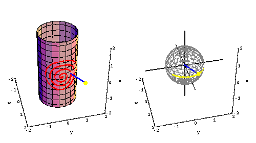
In the left graphic,
the cylinder surface x^2 + y^2 =1 is shown with
a
red curve on it.
This curve obtained by mapping the
unit circle
centered at the origin of the u-v plane to
the cylinder by the
parameterization
cyl[u,v] = {cos[u],sin[u],v}.
The blue
'outward'
unit normal with a yellow tip is shown at a
point
of this curve.
In the right graphic the blue
unit normal with
yellow
tip is shown translated to the origin,
with its
yellow
tip on a gray
sphere
(shown in wireframe view).The
yellow curve on the sphere is the image of
the red
curve under the
Gauss map of the cylinder. It consists of the image points
of the yellow
tips of the blue
unit
normals as the base points vary about the
red
curve.
Back to
Topics list.
Back to top.
Click on
the picture to see the animated view.
Or right click and choose "Save Target As" or "Save Link As"
here
to download a QuickTime movie (.mov file) of this animation. Picture/animation explanations:
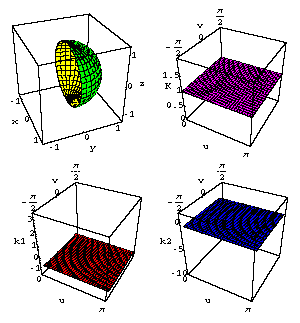
This graphic shows the first frame of
an animated view of the Theorema Egregium of Gauss, that
the (Gauss) curvature K of a surface
is invariant under isometry. The
green/yellow surface shown is a portion of the round sphere
of
radius 1. It is the starting surface in a family of isometric surfaces all of which
share the features of being surfaces of revolution with Gauss curvature K = 1 at every point.
To the right of the spherical surface is a purple graph of its Gauss curvature
as a
function of the sphere parameterization
variables { u , v } (the u-curves are mapped to the parallels,
the v-curves to meridians).
Below these are graphs of the principal
curvatures, k1 (red) and k2 (blue).
When the animation runs
the sphere portion varies through
the family of isometric surfaces.
The corresponding
principal curvature functions also vary, but the Gauss curvature, which is
given
by the product,
k1*k2 = K, remains constant. This exhibits the Theorema
Egregium in action.
Back to
Topics list.
Back to top.
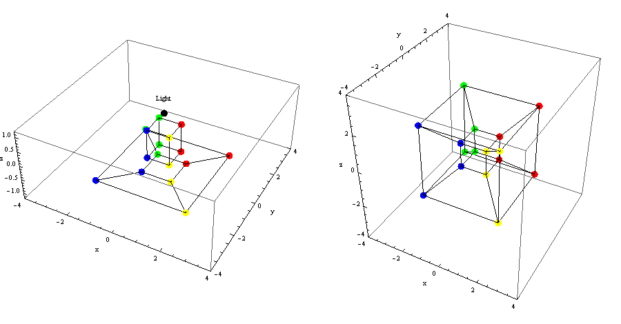
Click on
the picture to see the animated view.
Or right click and choose "Save Target As" or "Save Link As"
here
to download a QuickTime movie (.mov file) of this animation. Picture/animation explanations:
This graphic shows on the left the a rotating 3-d cube in three-space and its projection onto a 2-d plane below it.
There is a
black dot labeled "Light" which casts the "shadow" of the rotating cube (stereographic projection).
The vertices are color-coded so
they
and their projected images in the 2-d plane can be followed.
On the right we see the image of a 4-d cube projected onto a 3-d three-space
'below' it. Even though we
cannot see it or show a graphic for it, there is a
"Light" in four-space which casts the "shadow" of the rotating
4-d cube into three space.
The vertices are color-coded so
they and their projected images in the 3-d space can be followed.
Even though we cannot see the 4-space or the 4-d cube, we can still
see its "shadow" one dimension "down" in the
same way that we can see the 2-d image below
the rotating 3-d cube in three space.
Back to
Topics
list.
Back to top.
There
are lots of other Differential Geometry topics explored with
Mathematica and
Gray's programs in our courses.
The Mathematica notebooks are written
for an audience which I assume has NOT used Mathematica before.
The notebooks
were written so that students can
modify the input easily in order to examine
geometric attributes of different curves or
surfaces, or different points on given
curves and surfaces. These modifications are
included as exercises. I will be adding
further graphics and topics to those given
above in the future.
Please write me with
comments, suggestions,
corrections, ideas.... Please let me know if you would like me to
email any of the Mathematica files to you. Then you may modify them, use them however you want,
and let me know how to improve them!
Email address walter-seaman@uiowa.edu
Home page
http://www.math.uiowa.edu/~wseaman
Last updated April 26, 2015.
